评估扩散模型

生成模型（如Stable Diffusion）的评估本质上具有主观性。但作为从业者和研究人员，我们经常需要在众多不同的可能性中做出谨慎的选择。因此，在处理不同的生成模型（如GANs、Diffusion等）时，我们如何选择其中一个而不是另一个呢？

这类模型的定性评估可能容易出错，并可能错误地影响决策。然而，定量指标并不一定与图像质量相对应。因此，通常情况下，定性和定量评估的结合在选择模型时提供了更强的信号。

在本文件中，我们提供了一个非详尽的定性和定量方法概述，用于评估Diffusion模型。对于定量方法，我们特别关注如何与diffusers一起实现它们。

本文件中展示的方法也可以用于评估不同的噪声调度器，同时保持底层生成模型不变。

场景

我们涵盖了以下管道的Diffusion模型：

• 文本引导的图像生成（如StableDiffusionPipeline）。
• 文本引导的图像生成，额外基于输入图像的条件（如StableDiffusionImg2ImgPipeline和StableDiffusionInstructPix2PixPipeline）。
• 类别条件图像生成模型（如DiTPipeline）。

定性评估

定性评估通常涉及对生成图像的人类评估。质量通过构图、图像-文本对齐和空间关系等方面来衡量。常见的提示为主观指标提供了一定程度的一致性。DrawBench和PartiPrompts是用于定性基准测试的提示数据集。DrawBench和PartiPrompts分别由Imagen和Parti引入。

从官方Parti网站：

PartiPrompts（P2）是我们作为此工作的一部分发布的超过1600个英语提示的丰富集合。P2可用于衡量模型在各种类别和挑战方面的能力。

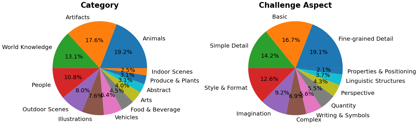
PartiPrompts包含以下列：

• 提示
• 提示的类别（如“抽象”、“世界知识”等）
• 反映难度的挑战（如“基本”、“复杂”、“书写与符号”等）

这些基准允许对不同的图像生成模型进行并排的人类评估。

为此，🧨 Diffusers团队构建了Open Parti Prompts，这是一个基于Parti Prompts的社区驱动的定性基准，用于比较最先进的开源扩散模型：

• Open Parti Prompts游戏：对于10个Parti提示，显示4张生成的图像，用户选择最适合提示的图像。
• Open Parti Prompts排行榜：比较当前最佳开源扩散模型之间的排行榜。

为了手动比较图像，让我们看看如何使用diffusers在几个PartiPrompts上进行操作。

下面我们展示了一些在不同挑战（基本、复杂、语言结构、想象和书写与符号）中采样的提示。这里我们使用PartiPrompts作为数据集。

from datasets import load_dataset

# prompts = load_dataset("nateraw/parti-prompts", split="train")
# prompts = prompts.shuffle()
# sample_prompts = [prompts[i]["Prompt"] for i in range(5)]

# Fixing these sample prompts in the interest of reproducibility.
sample_prompts = [
    "a corgi",
    "a hot air balloon with a yin-yang symbol, with the moon visible in the daytime sky",
    "a car with no windows",
    "a cube made of porcupine",
    'The saying "BE EXCELLENT TO EACH OTHER" written on a red brick wall with a graffiti image of a green alien wearing a tuxedo. A yellow fire hydrant is on a sidewalk in the foreground.',
]

现在我们可以使用这些提示来生成一些图像，使用的是Stable Diffusion（v1-4 checkpoint）：

import torch

seed = 0
generator = torch.manual_seed(seed)

images = sd_pipeline(sample_prompts, num_images_per_prompt=1, generator=generator).images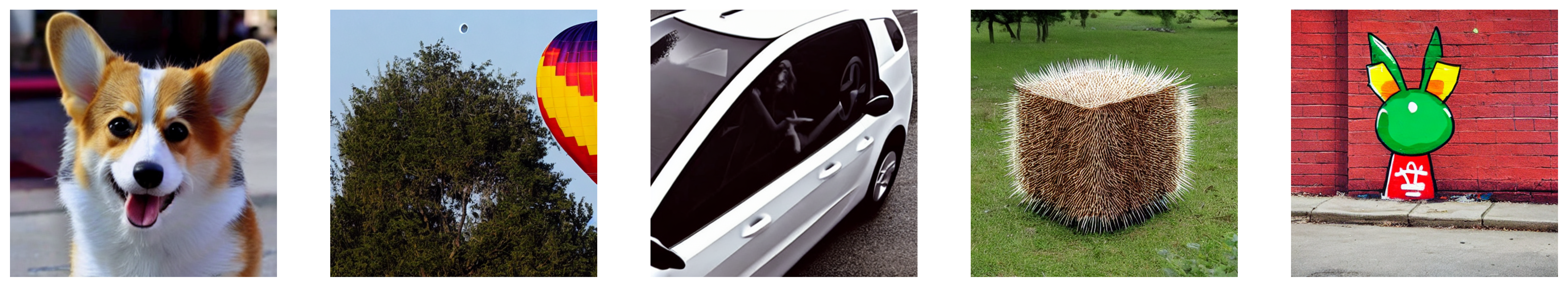

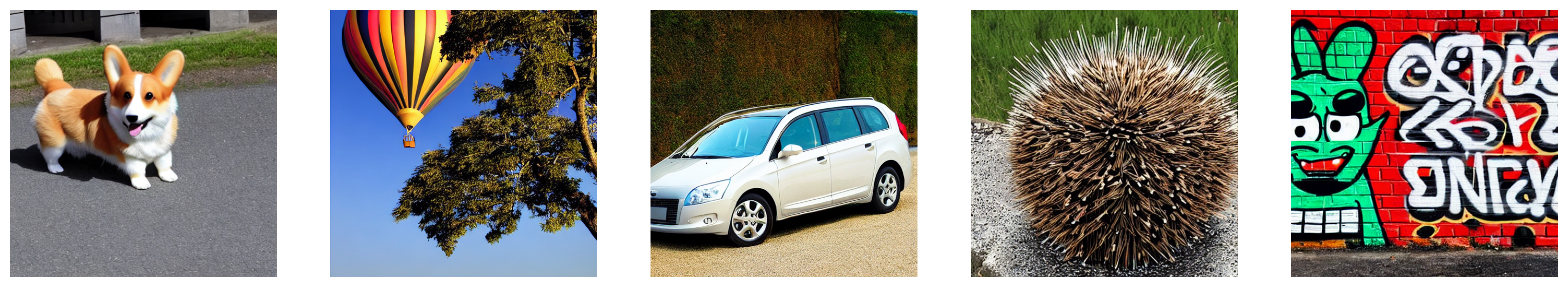
我们还可以相应地设置 num_images_per_prompt 来比较同一提示下的不同图像。运行相同的管道，但使用不同的检查点（v1-5），结果如下：

一旦使用多个模型（在评估中）从所有提示中生成了几张图像，这些结果就会呈现给人类评估者进行评分。有关 DrawBench 和 PartiPrompts 基准的更多详细信息，请参阅各自的论文。

定量评估

在本节中，我们将引导你了解如何使用以下方法评估三种不同的扩散管道：

• CLIP 分数
• CLIP 方向相似性
• FID

文本引导的图像生成

CLIP 分数 衡量图像-标题对的兼容性。更高的 CLIP 分数意味着更高的兼容性 🔼。CLIP 分数是对“兼容性”这一定性概念的定量测量。图像-标题对的兼容性也可以被认为是图像和标题之间的语义相似性。研究发现，CLIP 分数与人类判断具有高度相关性。

首先，让我们加载一个 [StableDiffusionPipeline]：

from diffusers import StableDiffusionPipeline
import torch

model_ckpt = "CompVis/stable-diffusion-v1-4"
sd_pipeline = StableDiffusionPipeline.from_pretrained(model_ckpt, torch_dtype=torch.float16).to("cuda")

生成一些带有多个提示的图像：

prompts = [
    "a photo of an astronaut riding a horse on mars",
    "A high tech solarpunk utopia in the Amazon rainforest",
    "A pikachu fine dining with a view to the Eiffel Tower",
    "A mecha robot in a favela in expressionist style",
    "an insect robot preparing a delicious meal",
    "A small cabin on top of a snowy mountain in the style of Disney, artstation",
]

images = sd_pipeline(prompts, num_images_per_prompt=1, output_type="np").images

print(images.shape)
# (6, 512, 512, 3)

然后，我们计算CLIP分数。

from torchmetrics.functional.multimodal import clip_score
from functools import partial

clip_score_fn = partial(clip_score, model_name_or_path="openai/clip-vit-base-patch16")

def calculate_clip_score(images, prompts):
    images_int = (images * 255).astype("uint8")
    clip_score = clip_score_fn(torch.from_numpy(images_int).permute(0, 3, 1, 2), prompts).detach()
    return round(float(clip_score), 4)

sd_clip_score = calculate_clip_score(images, prompts)
print(f"CLIP score: {sd_clip_score}")
# CLIP score: 35.7038

在上面的例子中，我们为每个提示生成了一个图像。如果我们为每个提示生成了多个图像，我们将不得不从每个提示生成的图像中取平均分数。

现在，如果我们想比较两个与[StableDiffusionPipeline]兼容的检查点，我们应该在调用管道时传递一个生成器。首先，我们使用v1-4 Stable Diffusion检查点生成带有固定种子的图像：

seed = 0
generator = torch.manual_seed(seed)

images = sd_pipeline(prompts, num_images_per_prompt=1, generator=generator, output_type="np").images

然后我们加载v1-5检查点来生成图像：

model_ckpt_1_5 = "stable-diffusion-v1-5/stable-diffusion-v1-5"
sd_pipeline_1_5 = StableDiffusionPipeline.from_pretrained(model_ckpt_1_5, torch_dtype=weight_dtype).to(device)

images_1_5 = sd_pipeline_1_5(prompts, num_images_per_prompt=1, generator=generator, output_type="np").images

最后，我们比较它们的CLIP分数：

sd_clip_score_1_4 = calculate_clip_score(images, prompts)
print(f"CLIP Score with v-1-4: {sd_clip_score_1_4}")
# CLIP Score with v-1-4: 34.9102

sd_clip_score_1_5 = calculate_clip_score(images_1_5, prompts)
print(f"CLIP Score with v-1-5: {sd_clip_score_1_5}")
# CLIP Score with v-1-5: 36.2137

看起来v1-5检查点比其前身表现更好。然而，需要注意的是，我们用于计算CLIP分数的提示数量相当少。为了进行更实际的评估，这个数量应该更高，并且提示应该多样化。

图像条件下的文本到图像生成

在这种情况下，我们使用输入图像和文本提示来条件生成管道。让我们以[StableDiffusionInstructPix2PixPipeline]为例。它接受一个编辑指令作为输入提示和一个要编辑的输入图像。

以下是一个示例：

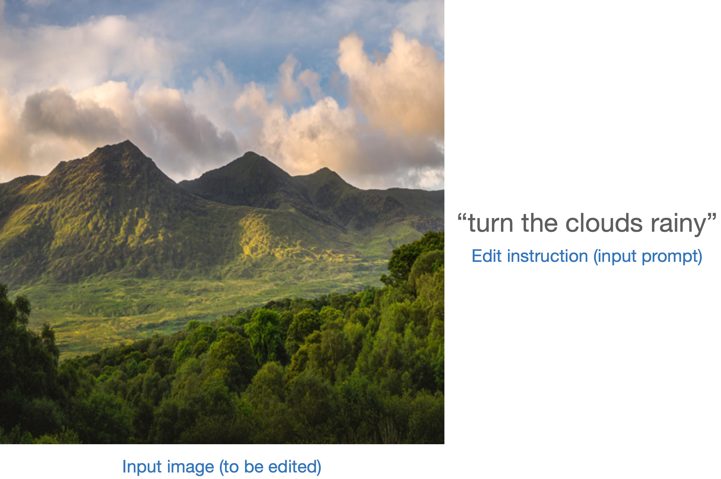
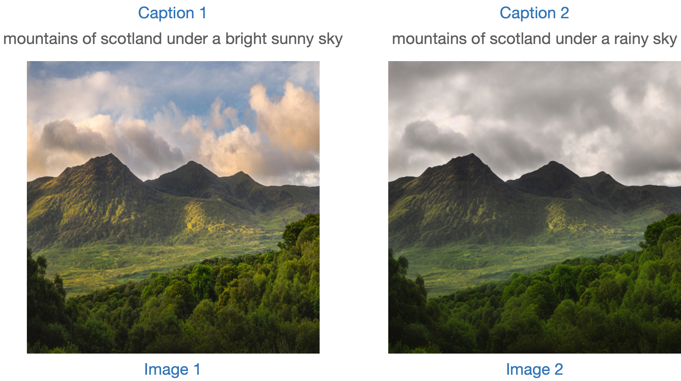
评估此类模型的一种策略是测量两张图像之间的变化（在CLIP空间中）与两张图像标题之间的变化（如CLIP引导的图像生成器领域适应所示）的一致性。这被称为“CLIP方向相似性”。

• 标题1对应于要编辑的输入图像（图像1）。
• 标题2对应于编辑后的图像（图像2）。它应反映编辑指令。

以下是图片概览：

我们已经准备了一个小型数据集来实现这一指标。首先加载数据集。

from datasets import load_dataset

dataset = load_dataset("sayakpaul/instructpix2pix-demo", split="train")
dataset.features

{'input': Value(dtype='string', id=None),
 'edit': Value(dtype='string', id=None),
 'output': Value(dtype='string', id=None),
 'image': Image(decode=True, id=None)}

这里我们有：

• input 是对应于 image 的标题。
• edit 表示编辑指令。
• output 表示反映 edit 指令的修改后的标题。

让我们来看一个示例。

idx = 0
print(f"Original caption: {dataset[idx]['input']}")
print(f"Edit instruction: {dataset[idx]['edit']}")
print(f"Modified caption: {dataset[idx]['output']}")

Original caption: 2. FAROE ISLANDS: An archipelago of 18 mountainous isles in the North Atlantic Ocean between Norway and Iceland, the Faroe Islands has 'everything you could hope for', according to Big 7 Travel. It boasts 'crystal clear waterfalls, rocky cliffs that seem to jut out of nowhere and velvety green hills'
Edit instruction: make the isles all white marble
Modified caption: 2. WHITE MARBLE ISLANDS: An archipelago of 18 mountainous white marble isles in the North Atlantic Ocean between Norway and Iceland, the White Marble Islands has 'everything you could hope for', according to Big 7 Travel. It boasts 'crystal clear waterfalls, rocky cliffs that seem to jut out of nowhere and velvety green hills'

这是图片：

dataset[idx]["image"]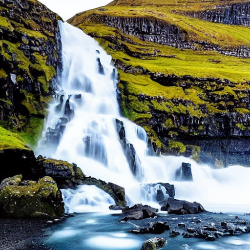

我们将首先使用编辑指令编辑数据集中的图像，并计算方向相似度。

首先，我们加载 [StableDiffusionInstructPix2PixPipeline]：

from diffusers import StableDiffusionInstructPix2PixPipeline

instruct_pix2pix_pipeline = StableDiffusionInstructPix2PixPipeline.from_pretrained(
    "timbrooks/instruct-pix2pix", torch_dtype=torch.float16
).to(device)

现在，我们执行编辑：

import numpy as np


def edit_image(input_image, instruction):
    image = instruct_pix2pix_pipeline(
        instruction,
        image=input_image,
        output_type="np",
        generator=generator,
    ).images[0]
    return image

input_images = []
original_captions = []
modified_captions = []
edited_images = []

for idx in range(len(dataset)):
    input_image = dataset[idx]["image"]
    edit_instruction = dataset[idx]["edit"]
    edited_image = edit_image(input_image, edit_instruction)

    input_images.append(np.array(input_image))
    original_captions.append(dataset[idx]["input"])
    modified_captions.append(dataset[idx]["output"])
    edited_images.append(edited_image)

为了测量方向相似度，我们首先加载 CLIP 的图像和文本编码器：

from transformers import (
    CLIPTokenizer,
    CLIPTextModelWithProjection,
    CLIPVisionModelWithProjection,
    CLIPImageProcessor,
)

clip_id = "openai/clip-vit-large-patch14"
tokenizer = CLIPTokenizer.from_pretrained(clip_id)
text_encoder = CLIPTextModelWithProjection.from_pretrained(clip_id).to(device)
image_processor = CLIPImageProcessor.from_pretrained(clip_id)
image_encoder = CLIPVisionModelWithProjection.from_pretrained(clip_id).to(device)

请注意，我们使用了一个特定的 CLIP 检查点，即 openai/clip-vit-large-patch14。这是因为 Stable Diffusion 的预训练是使用这个 CLIP 变体进行的。更多详情，请参阅 文档。

接下来，我们准备一个 PyTorch nn.Module 来计算方向相似度：

import torch.nn as nn
import torch.nn.functional as F


class DirectionalSimilarity(nn.Module):
    def __init__(self, tokenizer, text_encoder, image_processor, image_encoder):
        super().__init__()
        self.tokenizer = tokenizer
        self.text_encoder = text_encoder
        self.image_processor = image_processor
        self.image_encoder = image_encoder

    def preprocess_image(self, image):
        image = self.image_processor(image, return_tensors="pt")["pixel_values"]
        return {"pixel_values": image.to(device)}

    def tokenize_text(self, text):
        inputs = self.tokenizer(
            text,
            max_length=self.tokenizer.model_max_length,
            padding="max_length",
            truncation=True,
            return_tensors="pt",
        )
        return {"input_ids": inputs.input_ids.to(device)}

    def encode_image(self, image):
        preprocessed_image = self.preprocess_image(image)
        image_features = self.image_encoder(**preprocessed_image).image_embeds
        image_features = image_features / image_features.norm(dim=1, keepdim=True)
        return image_features

    def encode_text(self, text):
        tokenized_text = self.tokenize_text(text)
        text_features = self.text_encoder(**tokenized_text).text_embeds
        text_features = text_features / text_features.norm(dim=1, keepdim=True)
        return text_features

    def compute_directional_similarity(self, img_feat_one, img_feat_two, text_feat_one, text_feat_two):
        sim_direction = F.cosine_similarity(img_feat_two - img_feat_one, text_feat_two - text_feat_one)
        return sim_direction

    def forward(self, image_one, image_two, caption_one, caption_two):
        img_feat_one = self.encode_image(image_one)
        img_feat_two = self.encode_image(image_two)
        text_feat_one = self.encode_text(caption_one)
        text_feat_two = self.encode_text(caption_two)
        directional_similarity = self.compute_directional_similarity(
            img_feat_one, img_feat_two, text_feat_one, text_feat_two
        )
        return directional_similarity

现在让我们使用 DirectionalSimilarity。

dir_similarity = DirectionalSimilarity(tokenizer, text_encoder, image_processor, image_encoder)
scores = []

for i in range(len(input_images)):
    original_image = input_images[i]
    original_caption = original_captions[i]
    edited_image = edited_images[i]
    modified_caption = modified_captions[i]

    similarity_score = dir_similarity(original_image, edited_image, original_caption, modified_caption)
    scores.append(float(similarity_score.detach().cpu()))

print(f"CLIP directional similarity: {np.mean(scores)}")
# CLIP directional similarity: 0.0797976553440094

与CLIP分数类似，CLIP方向相似度越高越好。

需要注意的是，StableDiffusionInstructPix2PixPipeline 暴露了两个参数，即 image_guidance_scale 和 guidance_scale，让你可以控制最终编辑图像的质量。我们鼓励你尝试这两个参数，看看它们对方向相似度的影响。

我们可以将这一指标的概念扩展到测量原始图像和编辑版本之间的相似度。为此，我们可以直接进行 F.cosine_similarity(img_feat_two, img_feat_one)。对于这类编辑，我们仍然希望图像的主要语义尽可能保留，即相似度分数较高。

我们可以将这些指标用于类似的管道，例如 StableDiffusionPix2PixZeroPipeline。

当被评估的模型在大型图像字幕数据集（如LAION-5B数据集）上预训练时，扩展像IS、FID（稍后讨论）或KID这样的指标可能会很困难。这是因为这些指标的基础是一个在ImageNet-1k数据集上预训练的InceptionNet，用于提取中间图像特征。Stable Diffusion的预训练数据集与InceptionNet的预训练数据集可能重叠有限，因此在这里不适合用于特征提取。

使用上述指标有助于评估类条件模型。例如，DiT。它是在ImageNet-1k类上预训练的。

类条件图像生成

类条件生成模型通常在类标记数据集（如ImageNet-1k）上预训练。评估这些模型的流行指标包括Fréchet Inception Distance (FID)、Kernel Inception Distance (KID) 和 Inception Score (IS)。在本文件中，我们重点关注FID（Heusel et al.）。我们展示了如何使用DiTPipeline计算它，该管道在底层使用了DiT模型。

FID旨在测量两组图像数据集的相似度。根据此资源：

Fréchet Inception Distance 是两个图像数据集之间相似度的度量。研究表明，它与人类对视觉质量的判断有很好的相关性，并且最常用于评估生成对抗网络的样本质量。FID通过计算Inception网络特征表示拟合的两个高斯分布之间的Fréchet距离来计算。

这两个数据集本质上是真实图像数据集和假图像数据集（在我们的情况下是生成的图像）。FID通常使用两个大数据集计算。然而，对于本文档，我们将使用两个小数据集。

首先，让我们从ImageNet-1k训练集中下载一些图像：

from zipfile import ZipFile
import requests


def download(url, local_filepath):
    r = requests.get(url)
    with open(local_filepath, "wb") as f:
        f.write(r.content)
    return local_filepath

dummy_dataset_url = "https://hf.co/datasets/sayakpaul/sample-datasets/resolve/main/sample-imagenet-images.zip"
local_filepath = download(dummy_dataset_url, dummy_dataset_url.split("/")[-1])

with ZipFile(local_filepath, "r") as zipper:
    zipper.extractall(".")

from PIL import Image
import os

dataset_path = "sample-imagenet-images"
image_paths = sorted([os.path.join(dataset_path, x) for x in os.listdir(dataset_path)])

real_images = [np.array(Image.open(path).convert("RGB")) for path in image_paths]

以下是来自ImageNet-1k类别的10张图像："磁带播放器"、"链锯"（x2）、"教堂"、"加油站"（x3）、"降落伞"（x2）和"鲟鱼"。

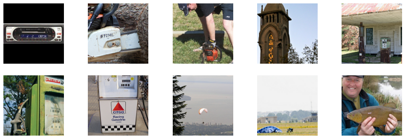
Real images.

现在图像已经加载完毕，让我们对它们进行一些轻量级的预处理，以便用于FID计算。

from torchvision.transforms import functional as F


def preprocess_image(image):
    image = torch.tensor(image).unsqueeze(0)
    image = image.permute(0, 3, 1, 2) / 255.0
    return F.center_crop(image, (256, 256))

real_images = torch.cat([preprocess_image(image) for image in real_images])
print(real_images.shape)
# torch.Size([10, 3, 256, 256])

我们现在加载 DiTPipeline 以根据上述类别生成图像。

from diffusers import DiTPipeline, DPMSolverMultistepScheduler

dit_pipeline = DiTPipeline.from_pretrained("facebook/DiT-XL-2-256", torch_dtype=torch.float16)
dit_pipeline.scheduler = DPMSolverMultistepScheduler.from_config(dit_pipeline.scheduler.config)
dit_pipeline = dit_pipeline.to("cuda")

words = [
    "cassette player",
    "chainsaw",
    "chainsaw",
    "church",
    "gas pump",
    "gas pump",
    "gas pump",
    "parachute",
    "parachute",
    "tench",
]

class_ids = dit_pipeline.get_label_ids(words)
output = dit_pipeline(class_labels=class_ids, generator=generator, output_type="np")

fake_images = output.images
fake_images = torch.tensor(fake_images)
fake_images = fake_images.permute(0, 3, 1, 2)
print(fake_images.shape)
# torch.Size([10, 3, 256, 256])

现在，我们可以使用 torchmetrics 计算FID。

from torchmetrics.image.fid import FrechetInceptionDistance

fid = FrechetInceptionDistance(normalize=True)
fid.update(real_images, real=True)
fid.update(fake_images, real=False)

print(f"FID: {float(fid.compute())}")
# FID: 177.7147216796875

FID 越低越好。以下几个因素会影响 FID：

• 图像数量（真实图像和生成图像）
• 扩散过程中引入的随机性
• 扩散过程中的推理步骤数量
• 扩散过程中使用的调度器

对于最后两点，因此，一个好的做法是在不同的种子和推理步骤下运行评估，然后报告平均结果。

最后一步，让我们直观地检查 fake_images。

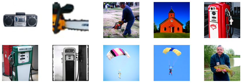
Fake images.