Marigold 管道用于计算机视觉任务

Marigold 是一种基于扩散的密集预测新方法，以及用于各种计算机视觉任务的一系列管道，例如单目深度估计。

本指南将向你展示如何使用 Marigold 获得图像和视频的快速且高质量的预测。

每个管道支持一个计算机视觉任务，该任务以输入的 RGB 图像作为输入，并生成感兴趣的模态的 预测，例如输入图像的深度图。 目前，已实现以下任务：

Pipeline	Predicted Modalities	Demos
MarigoldDepthPipeline	Depth, Disparity	Fast Demo (LCM), Slow Original Demo (DDIM)
MarigoldNormalsPipeline	Surface normals	Fast Demo (LCM)

原始检查点可以在 PRS-ETH Hugging Face 组织下找到。 这些检查点旨在与 diffusers 管道和 原始代码库 一起使用。 原始代码也可以用于训练新的检查点。

检查点	模态	注释
prs-eth/marigold-v1-0	深度	第一个 Marigold 深度检查点，用于预测 仿射不变深度 地图。该检查点在基准测试中的性能在原始 论文 中进行了研究。设计用于在推理时与 DDIMScheduler 一起使用，至少需要 10 步才能获得可靠的预测。仿射不变深度预测的每个像素值范围在 0（近平面）到 1（远平面）之间；这两个平面由模型在推理过程中选择。请参阅 MarigoldImageProcessor 参考以获取可视化工具。
prs-eth/marigold-depth-lcm-v1-0	深度	快速 Marigold 深度检查点，从 prs-eth/marigold-v1-0 微调而来。设计用于在推理时与 LCMScheduler 一起使用，最少需要 1 步即可获得可靠的预测。预测可靠性在 4 步时达到饱和，之后会下降。
prs-eth/marigold-normals-v0-1	法线	Marigold 法线管道的预览检查点。设计用于在推理时与 DDIMScheduler 一起使用，至少需要 10 步才能获得可靠的预测。表面法线预测是单位长度的 3D 向量，值范围从 -1 到 1。此检查点将在 v1-0 版本发布后逐步淘汰。
prs-eth/marigold-normals-lcm-v0-1	法线	快速 Marigold 法线检查点，从 prs-eth/marigold-normals-v0-1 微调而来。设计用于在推理时与 LCMScheduler 一起使用，最少需要 1 步即可获得可靠的预测。预测可靠性在 4 步时达到饱和，之后会下降。此检查点将在 v1-0 版本发布后逐步淘汰。

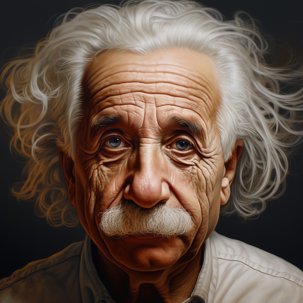
以下示例主要针对深度预测，但它们可以普遍应用于其他支持的模态。 我们使用 Midjourney 生成的同一张爱因斯坦输入图像来展示预测结果。 这使得在各种模态和检查点之间比较预测的可视化结果更加容易。

Example input image for all Marigold pipelines

深度预测快速入门

要获得第一个深度预测，将 prs-eth/marigold-depth-lcm-v1-0 检查点加载到 MarigoldDepthPipeline 管道中，将图像通过管道处理，并保存预测结果：

import diffusers
import torch

pipe = diffusers.MarigoldDepthPipeline.from_pretrained(
    "prs-eth/marigold-depth-lcm-v1-0", variant="fp16", torch_dtype=torch.float16
).to("cuda")

image = diffusers.utils.load_image("https://marigoldmonodepth.github.io/images/einstein.jpg")
depth = pipe(image)

vis = pipe.image_processor.visualize_depth(depth.prediction)
vis[0].save("einstein_depth.png")

depth_16bit = pipe.image_processor.export_depth_to_16bit_png(depth.prediction)
depth_16bit[0].save("einstein_depth_16bit.png")

深度可视化功能 [~pipelines.marigold.marigold_image_processing.MarigoldImageProcessor.visualize_depth] 将 matplotlib 的颜色映射（默认为 Spectral）应用于将单通道 [0, 1] 深度范围内的预测像素值映射为 RGB 图像。 使用 Spectral 颜色映射时，近处的像素会被涂成红色，远处的像素会被赋予蓝色。 16 位 PNG 文件将单通道值从 [0, 1] 范围线性映射到 [0, 65535]。 以下是原始预测和可视化预测；可以看到，暗区（如胡须）在可视化中更容易区分：

Predicted depth (16-bit PNG)

Predicted depth visualization (Spectral)

表面法线预测快速入门

将 prs-eth/marigold-normals-lcm-v0-1 检查点加载到 MarigoldNormalsPipeline 管道中，将图像通过管道处理，并保存预测结果：

import diffusers
import torch

pipe = diffusers.MarigoldNormalsPipeline.from_pretrained(
    "prs-eth/marigold-normals-lcm-v0-1", variant="fp16", torch_dtype=torch.float16
).to("cuda")

image = diffusers.utils.load_image("https://marigoldmonodepth.github.io/images/einstein.jpg")
normals = pipe(image)

vis = pipe.image_processor.visualize_normals(normals.prediction)
vis[0].save("einstein_normals.png")

可视化函数 [~pipelines.marigold.marigold_image_processing.MarigoldImageProcessor.visualize_normals] 将范围在 [-1, 1] 的三维预测值映射为 RGB 图像。 该可视化函数支持翻转表面法线轴，以使可视化结果与其他参考系的选择兼容。 概念上，每个像素根据参考系中的表面法线向量进行着色，其中 X 轴指向右侧，Y 轴指向上方，Z 轴指向观察者。 以下是可视化的预测结果：

Predicted surface normals visualization

在这个例子中，鼻尖几乎肯定有一个表面点，其表面法向量直接指向观察者，这意味着其坐标为 [0, 0, 1]。 这个向量映射到 RGB [128, 128, 255]，对应于蓝紫色。 同样，图像右侧脸颊上的表面法向量具有较大的 X 分量，这会增加红色调。 指向上的肩膀上的点具有较大的 Y 分量，会促进绿色的出现。

加速推理

上述快速入门代码片段已经针对速度进行了优化：它们加载了 LCM 检查点，使用 fp16 权重和计算变体，并且只执行一次去噪扩散步骤。 在 RTX 3090 GPU 上，pipe(image) 调用在 280 毫秒内完成。 内部，输入图像首先通过 Stable Diffusion VAE 编码器进行编码，然后 U-Net 执行一次去噪步骤，最后预测的潜在变量通过 VAE 解码器解码到像素空间。 在这种情况下，三个模块调用中有两个专门用于在 LDM 的像素空间和潜在空间之间进行转换。 由于 Marigold 的潜在空间与基础 Stable Diffusion 兼容，通过使用 SD VAE 的轻量级替代品，可以将管道调用加速超过 3 倍（在 RTX 3090 上为 85 毫秒）。

  import diffusers
  import torch

  pipe = diffusers.MarigoldDepthPipeline.from_pretrained(
      "prs-eth/marigold-depth-lcm-v1-0", variant="fp16", torch_dtype=torch.float16
  ).to("cuda")

+ pipe.vae = diffusers.AutoencoderTiny.from_pretrained(
+     "madebyollin/taesd", torch_dtype=torch.float16
+ ).cuda()

  image = diffusers.utils.load_image("https://marigoldmonodepth.github.io/images/einstein.jpg")
  depth = pipe(image)

正如在 优化 中建议的，添加 torch.compile 可能会根据目标硬件挤出额外的性能：

  import diffusers
  import torch

  pipe = diffusers.MarigoldDepthPipeline.from_pretrained(
      "prs-eth/marigold-depth-lcm-v1-0", variant="fp16", torch_dtype=torch.float16
  ).to("cuda")

+ pipe.unet = torch.compile(pipe.unet, mode="reduce-overhead", fullgraph=True)

  image = diffusers.utils.load_image("https://marigoldmonodepth.github.io/images/einstein.jpg")
  depth = pipe(image)

与 Depth Anything 的定性比较

通过上述速度优化，Marigold 在使用最大的检查点 LiheYoung/depth-anything-large-hf 时，比 Depth Anything 提供了更多细节且速度更快：

Marigold LCM fp16 with Tiny AutoEncoder

Depth Anything Large

最大化精度和集成

Marigold 管道内置了一种集成机制，结合了来自不同随机潜在变量的多个预测。 这是一种通过利用扩散的生成性质来提高预测精度的暴力方法。 当 ensemble_size 参数设置为大于 1 时，集成路径会自动激活。 在追求最大精度时，同时调整 num_inference_steps 和 ensemble_size 是合理的。 推荐的值因检查点而异，但主要取决于调度器类型。 集成的效果在表面法线方面尤为明显。

import diffusers

model_path = "prs-eth/marigold-normals-v1-0"

model_paper_kwargs = {
	diffusers.schedulers.DDIMScheduler: {
		"num_inference_steps": 10,
		"ensemble_size": 10,
	},
	diffusers.schedulers.LCMScheduler: {
		"num_inference_steps": 4,
		"ensemble_size": 5,
	},
}

image = diffusers.utils.load_image("https://marigoldmonodepth.github.io/images/einstein.jpg")

pipe = diffusers.MarigoldNormalsPipeline.from_pretrained(model_path).to("cuda")
pipe_kwargs = model_paper_kwargs[type(pipe.scheduler)]

depth = pipe(image, **pipe_kwargs)

vis = pipe.image_processor.visualize_normals(depth.prediction)
vis[0].save("einstein_normals.png")

Surface normals, no ensembling

Surface normals, with ensembling

可以看到，所有具有细粒度结构的区域，如头发，都得到了更加保守且平均更准确的预测。 这样的结果更适合对精度敏感的下游任务，如3D重建。

定量评估

为了在标准排行榜和基准测试（如NYU、KITTI和其他数据集）中对Marigold进行定量评估，请遵循论文中概述的评估协议：加载全精度fp32模型，并使用适当的num_inference_steps和ensemble_size值。 可选地设置随机种子以确保可重复性。最大化batch_size将实现设备的最大利用率。

import diffusers
import torch

device = "cuda"
seed = 2024
model_path = "prs-eth/marigold-v1-0"

model_paper_kwargs = {
	diffusers.schedulers.DDIMScheduler: {
		"num_inference_steps": 50,
		"ensemble_size": 10,
	},
	diffusers.schedulers.LCMScheduler: {
		"num_inference_steps": 4,
		"ensemble_size": 10,
	},
}

image = diffusers.utils.load_image("https://marigoldmonodepth.github.io/images/einstein.jpg")

generator = torch.Generator(device=device).manual_seed(seed)
pipe = diffusers.MarigoldDepthPipeline.from_pretrained(model_path).to(device)
pipe_kwargs = model_paper_kwargs[type(pipe.scheduler)]

depth = pipe(image, generator=generator, **pipe_kwargs)

# evaluate metrics

使用预测不确定性

Marigold 管道中内置的集成机制结合了从不同随机潜在变量获得的多个预测。 作为副作用，它可以用于量化认识不确定性（模型不确定性）；只需将 ensemble_size 设置为大于 1 并将 output_uncertainty 设置为 True。 生成的不确定性将在输出的 uncertainty 字段中可用。 它可以如下可视化：

import diffusers
import torch

pipe = diffusers.MarigoldDepthPipeline.from_pretrained(
    "prs-eth/marigold-depth-lcm-v1-0", variant="fp16", torch_dtype=torch.float16
).to("cuda")

image = diffusers.utils.load_image("https://marigoldmonodepth.github.io/images/einstein.jpg")
depth = pipe(
	image,
	ensemble_size=10,  # any number greater than 1; higher values yield higher precision
	output_uncertainty=True,
)

uncertainty = pipe.image_processor.visualize_uncertainty(depth.uncertainty)
uncertainty[0].save("einstein_depth_uncertainty.png")

Depth uncertainty

Surface normals uncertainty

不确定性解释起来很简单：较高的值（白色）对应于模型难以做出一致预测的像素。 显然，深度模型在边缘不连续处（即物体深度急剧变化的地方）最不自信。 表面法线模型在细粒度结构（如头发）和暗区域（如衣领）处最不自信。

帧间视频处理与时间一致性

由于 Marigold 的生成性质，每个预测都是独特的，并由用于潜在初始化的随机噪声定义。 这与传统的端到端密集回归网络相比成为一个明显的缺点，如下视频所示：

Input video

Marigold Depth applied to input video frames independently

为了解决这个问题，可以将 latents 参数传递给管道，该参数定义了扩散的起点。 通过实验，我们发现，将相同的起始点噪声潜在变量与前一帧预测对应的潜在变量进行凸组合，可以得到足够平滑的结果，如下代码片段所示：

import imageio
from PIL import Image
from tqdm import tqdm
import diffusers
import torch

device = "cuda"
path_in = "obama.mp4"
path_out = "obama_depth.gif"

pipe = diffusers.MarigoldDepthPipeline.from_pretrained(
    "prs-eth/marigold-depth-lcm-v1-0", variant="fp16", torch_dtype=torch.float16
).to(device)
pipe.vae = diffusers.AutoencoderTiny.from_pretrained(
    "madebyollin/taesd", torch_dtype=torch.float16
).to(device)
pipe.set_progress_bar_config(disable=True)

with imageio.get_reader(path_in) as reader:
    size = reader.get_meta_data()['size']
    last_frame_latent = None
    latent_common = torch.randn(
        (1, 4, 768 * size[1] // (8 * max(size)), 768 * size[0] // (8 * max(size)))
    ).to(device=device, dtype=torch.float16)

    out = []
    for frame_id, frame in tqdm(enumerate(reader), desc="Processing Video"):
        frame = Image.fromarray(frame)
        latents = latent_common
        if last_frame_latent is not None:
            latents = 0.9 * latents + 0.1 * last_frame_latent

        depth = pipe(
			frame, match_input_resolution=False, latents=latents, output_latent=True
        )
        last_frame_latent = depth.latent
        out.append(pipe.image_processor.visualize_depth(depth.prediction)[0])

    diffusers.utils.export_to_gif(out, path_out, fps=reader.get_meta_data()['fps'])

在这里，扩散过程从给定的计算潜在变量开始。 管道设置 output_latent=True 以访问 out.latent 并计算其对下一帧潜在变量初始化的贡献。 现在结果更加稳定了：

Marigold Depth applied to input video frames independently

Marigold Depth with forced latents initialization

Marigold 用于 ControlNet

深度预测与扩散模型结合的常见应用之一是与 ControlNet 一起使用。 深度清晰度在从 ControlNet 获得高质量结果中起着关键作用。 如上所述与其他方法的比较所示，Marigold 在此任务中表现出色。 以下代码片段展示了如何加载图像、计算深度，并将其以兼容格式传递给 ControlNet：

import torch
import diffusers

device = "cuda"
generator = torch.Generator(device=device).manual_seed(2024)
image = diffusers.utils.load_image(
    "https://huggingface.co/datasets/huggingface/documentation-images/resolve/main/diffusers/controlnet_depth_source.png"
)

pipe = diffusers.MarigoldDepthPipeline.from_pretrained(
    "prs-eth/marigold-depth-lcm-v1-0", torch_dtype=torch.float16, variant="fp16"
).to(device)

depth_image = pipe(image, generator=generator).prediction
depth_image = pipe.image_processor.visualize_depth(depth_image, color_map="binary")
depth_image[0].save("motorcycle_controlnet_depth.png")

controlnet = diffusers.ControlNetModel.from_pretrained(
    "diffusers/controlnet-depth-sdxl-1.0", torch_dtype=torch.float16, variant="fp16"
).to(device)
pipe = diffusers.StableDiffusionXLControlNetPipeline.from_pretrained(
    "SG161222/RealVisXL_V4.0", torch_dtype=torch.float16, variant="fp16", controlnet=controlnet
).to(device)
pipe.scheduler = diffusers.DPMSolverMultistepScheduler.from_config(pipe.scheduler.config, use_karras_sigmas=True)

controlnet_out = pipe(
    prompt="high quality photo of a sports bike, city",
    negative_prompt="",
    guidance_scale=6.5,
    num_inference_steps=25,
    image=depth_image,
    controlnet_conditioning_scale=0.7,
    control_guidance_end=0.7,
    generator=generator,
).images
controlnet_out[0].save("motorcycle_controlnet_out.png")

Input image

Depth in the format compatible with ControlNet

ControlNet generation, conditioned on depth and prompt: "high quality photo of a sports bike, city"

希望你发现 Marigold 在解决你的下游任务时非常有用，无论是作为更广泛的生成工作流的一部分，还是感知任务，如 3D 重建。